Ambient Occlusion Fields

Recently I created a new example that we added to the online editor: a simple showcase using ambient occlusion fields. This is a lightweight method to approximate ambient occlusion in real time using a 3D lookup table.

There is no single best method for calculating ambient occlusion, because various approaches shine under different conditions. For instance, screen-space methods are more likely to perform better when shading (very) small features, while working at the scale of objects or rooms requires solutions that work in world space, unless the artistic intent calls for a deliberately unrealistic look. VR applications especially favour world-space effects due to the increased need for temporal and spatial coherence.

I was interested in finding a reasonable approximation of ambient occlusion by big moving objects without unpleasant temporal artifacts, so it was clear from the beginning that a screen-space postprocessing effect was out of the question. I also ruled out approaches based on raymarching and raytracing, because I wanted it to be lightweight enough for mobile and other low-performance devices, and support any possible occluder shape defined as a triangle mesh. Being physically accurate was less of a concern for me as long as the result looked convincing.

First of all, I did a little research on world-space methods. I quickly found two solutions that are the most widely cited:

1. Ambient Occlusion Fields by Kontkanen and Laine, which uses a cube map to encode the occlusion by a single object. Each entry of the map contains coefficients for an approximation function that returns the occlusion term given the distance from the centre of the object in the direction corresponding to the entry. They also describe a way to combine the occlusion terms originating from several objects by exploiting blending.
2. Ambient Occlusion Fields and Decals in Infamous 2, which is a more direct approach that stores occlusion information (amount and general direction) in a 3D texture fitted around the casting object. This allows a more accurate reconstruction of occlusion, especially close to or within the convex hull of the object, at the cost of higher memory requirements.

I thought the latter approach was promising and created a prototype implementation. However, I was unhappy with the results exactly where I expected this method to shine: inside and near the the object, and especially when it should have been self-shadowing.

After exhausting my patience for hacks, I had a different idea: instead of storing the general direction and strength of the occlusion at every sampling point, I’d directly store the strength in each of the six principal (axis-aligned) directions. The results surpassed all my expectations! The shading effect was very well-behaved and robust in general, and all the issues with missing occlusion went away instantly. While this meant increasing the number of terms from 4 to 6 for each sample, thanks to the improved behaviour the sampling resolution could be reduced enough to more than make up for it – consider that decreasing resolution by only 20% is enough to nearly halve the volume.

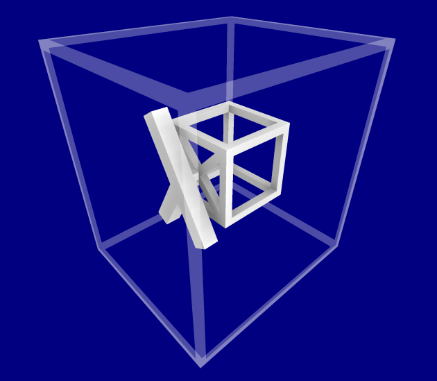
The real beef of this method is in the preprocessing step to generate the field, so let’s go through the process step by step. First of all, we take the bounding box of the object and add some padding to capture the domain where we want the approximation to work:

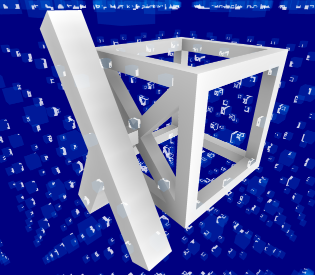
Next, we sample occlusion at every point by rendering the object on an 8×8 cube map as seen from that point. We just want a black and white image where the occluded parts are white. There is no real need for higher resolution or antialiasing, as we’ll have more than 256 samples affecting each of the final terms. Here’s how the cube maps look like (using 10x10x10 sampling points for the illustration):

Now we need a way to reduce each cube map to just six occlusion terms, one for each of the principal directions. The obvious thing to do is to define them as averages over half cubes. E.g. the up term is an average of the upper half of the cube, the right term is derived from the right half etc. For better accuracy, it might help to weight the samples of the cube map based on the relative directions they represent, but I chose not to do this because I was satisfied with the outcome even with simple averaging, and the difference is unlikely to be significant. Your mileage may vary.

The resulting terms can be stored in two RGB texels per sample, either in a 3D texture or a 2D one if your target platform has no support for the former (looking at you, WebGL).

To recap, here’s the whole field generation process in pseudocode:

principal_directions = {left, down, back, right, up, forward}
for each sample_index in (1, 1, 1) to (x_res, y_res, z_res)
   pos = position of the grid point at sample_index
   sample = black and white 8x8 cube map capture of object at pos
   for each dir_index in 1 to 6
      dir = principal_directions[dir_index]
      hemisphere = all texels of sample in the directions at acute angle with dir
      terms[dir_index] = average(hemisphere)
   field_negative[sample_index] = (r: terms[1], g: terms[2], b: terms[3])
   field_positive[sample_index] = (r: terms[4], g: terms[5], b: terms[6])

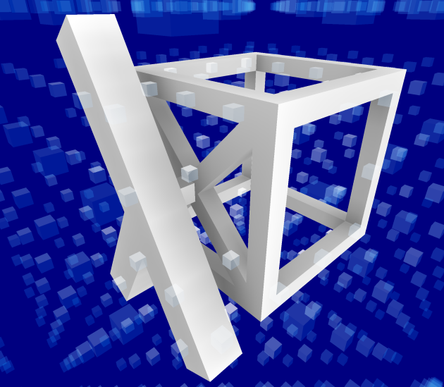
This is what it looks like when sampling at a resolution of 32x32x32 (negative XYZ terms on top, positive XYZ terms on bottom):

The resulting image is basically a voxelised representation of the object. Given this data, it is very easy to extract the final occlusion term during rendering. The key equation is the following:

occlusion = dot(minField(p), max(-n, 0)) + dot(maxField(p), max(n, 0)), where

• p = the position of the sampling point in field space (this is normalised, i.e. (0,0,0) corresponds to one corner of the original bounding box used to generate the samples, and (1,1,1) covers the opposite corner)
• n = the normal of the surface in occluder local space
• minField = function to sample the minimum/negative terms (a single texture lookup if we have a 3D texture, two lookups and a lerp if we have a 2D texture)
• maxField = function to sample the maximum/positive terms

All we’re doing here is computing a weighted sum of the occlusion terms, where the weights are the clamped dot products of n with the six principal directions. These weights happen to be the same as the individual components of the normal, so instead of doing six dot products, we can get them by zeroing out the negative terms of n and -n.
Putting aside the details of obtaining p and n for a moment, let’s look at the result. Not very surprisingly, the ambient term computed from the above field suffers from aliasing, which is especially visible when moving the object. Blurring the field with an appropriate kernel before use can completely eliminate this artifact. I settled with the following 3x3x3 kernel:

1	4	1		4	9	4		1	4	1
4	9	4		9	16	9		4	9	4
1	4	1		4	9	4		1	4	1

Also, since the field is finite in size, I decided to simply fade out the terms to zero near the edge to improve the transition at the boundary. In the Infamous 2 implementation they opted for remapping the samples so the highest boundary value would be zero, but this means that every object has a different mapping that needs to be fixed with other magic coefficients later on. Here’s a comparison of the original (left) and the blurred (right) fields:

Back to the problem of sampling. Most of the work is just transforming points and vectors between coordinate systems, so it can be done in the vertex shader. Let’s define a few transformations:

• F – occluder local to (normalised) field space, i.e. map the bounding box in the occluder’s local space to the range (0,0,0)-(1,1,1); this matrix is tied to the baked field, therefore it’s constant
• O – occluder local to world space, i.e. occluder model transformation
• R – receiver local to world space, i.e. receiver model transformation

I’ll use the f, o, and r subscripts to denote that a point or vector is in field, occluder local or receiver local space, e.g. p_f is the field space position, or n_r is the receiver’s local surface normal. When rendering an occluder, our constant input is F, O, R, and per vertex input is p_r and n_r. Given this data, we can now derive the values of p and n needed for sampling:

n = n_o = normalize(O^-1 * R * n_r)
p = p_f + n * bias = F * O^-1 * R * p_r + n * bias

The bias factor is the inversely proportional to the field’s resolution (I’m using 1/32 in the example, but it could also be a non-uniform scale if the field is not cube shaped), and its role is to prevent surfaces from shadowing themselves. Note that we’re not transforming the normal into field space, since that would alter its direction.

And that’s pretty much it! So far I’m very pleased with the results. One improvement I believe might be worth looking into is reducing the amount of terms from 6 to 4 per sample, so we can halve the amount of texture space and lookups needed. To do this, I’d pick the normals of a regular tetrahedron instead of the six principal directions for reference, and compute 4 dot products in the vertex shader (the 4 reference normals could be packed in a 4×3 matrix N) to determine the contribution of each term:

weights = N * n_o = (dot(n_o, n₁), dot(n_o, n₂), dot(n_o, n₃), dot(n_o, n₄))
occlusion = dot(field(p), max(weights, 0))

As soon as LambdaCube is in a good shape again, I’m planning to augment our beloved Stunts example with this effect.

Tuples as heterogeneous lists

You probably know that lists and tuples are in no way special data types in Haskell. They are basically the following ADTs (algebraic data types) with special syntax:

data List a           -- syntax in type context:        [a]
    = Nil             -- syntax in expression context:  []
    | Cons a (List a) -- syntax in expression context:  (a : as)

data Tuple2 a b       -- syntax in type context:        (a, b)
    = Tuple2 a b      -- syntax in expression context:  (a, b)

data Tuple3 a b c     -- syntax in type context:        (a, b, c)
    = Tuple3 a b c    -- syntax in expression context:  (a, b, c)

data Tuple4 a b c d   -- syntax in type context:        (a, b, c, d)
    = Tuple4 a b c d  -- syntax in expression context:  (a, b, c, d)

...

All right, but what exactly does that ... mean at the end? Do infinite tuples exist? Or at least, are there infinitely many tuples with different arities? In the case of GHC the answer is no, and this is very easy to demonstrate. Try to enter this tuple in ghci:

GHCi, version 7.10.3: http://www.haskell.org/ghc/ :? for help
Prelude> (0,0,0,0,0,0,0,0,0,0,0,0,0,0,0,0,0,0,0,0,0,0,0,0,0,0,0,0,0,0,0,0,0,0,0,0,0,0,0,0,0,0,0,0,0,0,0,0,0,0,0,0,0,0,0,0,0,0,0,0,0,0,0)
<interactive>:2:1:
    A 63-tuple is too large for GHC
      (max size is 62)
      Workaround: use nested tuples or define a data type

Although this seems reasonable, those who strive for perfection are not satisfied. What is the right solution for this problem? What is the real problem by the way?

I consider the Tuple2, Tuple3, Tuple4, … ADT family an inferior representation of tuples because of the following reasons:

1. There is this ugly … at the end with several consequences.
2. This family has no proper beginning. We can define both Tuple0 and Tuple1, but one-element tuples are not yet embraced by the Haskell community.
3. Tuples with different arities are not related to each other, because they are defined separately, not at once as one data family. One consequence of this is that it is not possible to write generic functions for tuples.

What would be a better representation of tuples? Heterogeneous lists, of course!

data HList :: List Type -> Type where
    HNil  :: HList 'Nil
    HCons :: forall t ts . t -> HList ts -> HList ('Cons t ts)

Some examples:

    HNil                      ::  HList 'Nil
    HCons True HNil           ::  HList ('Cons Bool 'Nil)
    HCons 3 (HCons True HNil) ::  HList ('Cons Int ('Cons Bool 'Nil)

The syntactic sugar for heterogeneous lists could be the same as for tuples, for example

    ()          ==> HNil                                -- in expression context
    ()          ==> HList 'Nil                          -- in type context
    (3, True)   ==> HCons 3 (HCons True HNil)           -- in expression context
    (Int, Bool) ==> HList ('Cons Int ('Cons Bool 'Nil)  -- in type context

What are the issues of representing tuples by heterogeneous lists?

1. There is a thing called one-element tuple, which needs explicit syntax.
2. We need some type system extensions (at least GADTs and type level lists are needed).
3. The compiler backend has to be a little bit smarter to produce efficient code for tuples.
4. Pattern matching on tuples is not obvious anymore.

The LambaCube 3D compiler solves the above issues the following way:

1. One element tuples are denoted by (( element )).
2. The compiler has a dependently typed core language, therefore defining and using the HList data type works out-of-the-box.
3. Currently the compiler has no code generator for CPUs and it has only a limited code generator for GPUs with no support for tuples. Tuples either vanish during reduction, or they are transformed away in the shader code generator.
4. Pattern matching on heterogeneous lists is restricted: when a tuple is matched, all patterns should have the same tuple arity. We’re okay with this, since this behaviour is not surprising for most programmers, and in LambdaCube 3D code tuple patterns tend to appear without alternative choices anyway.

After solving these issues, and migrating to the new representation of tuples, the built-in LambdaCube 3D library could be simplified significantly.

Some examples: previously we had repetitive, incomplete and potentially wrong functions for tuples like

type family JoinTupleType t1 t2 where
    JoinTupleType a () = a
    JoinTupleType a (b, c) = (a, b, c)
    JoinTupleType a (b, c, d) = (a, b, c, d)
    JoinTupleType a (b, c, d, e) = (a, b, c, d, e)
    JoinTupleType a b = (a, b)  -- this is wrong if b is a 5-tuple!
    -- JoinTupleType a ((b)) = (a, b)  -- something like this would be OK

remSemantics :: ImageSemantics -> Type
remSemantics = ... -- definition is not relevant now

remSemantics_ :: [ImageSemantics] -> Type
remSemantics_ [] = '()
remSemantics_ [a] = remSemantics a -- not good enough...
-- remSemantics_ [a] = '((remSemantics a))  -- something like this would be OK
remSemantics_ [a, b] = '(remSemantics a, remSemantics b)
remSemantics_ [a, b, c] = '(remSemantics a, remSemantics b, remSemantics c)
remSemantics_ [a, b, c, d] = '(remSemantics a, remSemantics b, remSemantics c, remSemantics d)
remSemantics_ [a, b, c, d, e] = '(remSemantics a, remSemantics b, remSemantics c, remSemantics d, remSemantics e)

With heterogeneous lists as tuples these and similar functions shrank considerably:

type family JoinTupleType a b where
    JoinTupleType x (HList xs) = HList '(x: xs)

remSemantics_ :: [ImageSemantics] -> Type
remSemantics_ ts = 'HList (map remSemantics ts)

By the way, with heterogeneous lists it was also easier to add row polymorphism (one solution for generic records) to the type system, but that is a different story.

The pattern matching issue deserves a bit more detail. Why is it a good idea to restrict pattern matching for heterogeneous lists? Well, consider the following function with no type annotation:

swap (a, b) = (b, a)

Of course we expect the compiler to infer the type of swap. On the other hand, if tuples are heterogeneous lists, the following function is also typeable:

f (_, _) = 2
f (_, _, _) = 3
f _ = 0

It seems that type inference is not feasible for heterogeneous lists in general. For LambdaCube 3D we settled with above mentioned restriction in order to retain type inference. It seems feasible to create a system that allows the definition of f with a type annotation, but this would not buy much for the users of LambdaCube 3D so we didn’t go for it.

I have found a few implementations of heterogeneous lists in Haskell, Idris and Agda. So far I have not found a language where tuples are represented with heterogeneous lists, neither a language with special syntax for heterogeneous lists.

1. HVect in reroute package is the same as HList.
2. HVect in hvect package is a strict variant of HList.
3. Tuples in Idris are different: (x, y, z) is a synonym for (x, (y, z)). On the other hand, HVect in the standard library is similar to HList. The difference is that the type level list is indexed by its length. I have found this discussion about whether tuples could be represented with HVect. It seems that efficient code generation is the difficult part.
4. I have found an implementation of HList and HVec in Agda. However, I also found this discussion about size problems, so it is not so convenient to use them. We don’t have such issues because we use type-in-type.
5. https://wiki.haskell.org/Heterogenous_collections gives a summary about implementing heterogeneous collections in Haskell. Heterogeneous lists are at the bottom (see next item).
6. Strongly typed heterogeneous collections by Oleg Kiselyov has a more complicated implementation of heterogeneous lists in Haskell using less type system extensions.

To sum it up, in the case of LambdaCube 3D, representing tuples as heterogeneous lists has no drawback and at the same time the base library (which provides the OpenGL binding) became more complete, shorter and more correct. We definitely consider switching to this representation an overall win.

Version 0.5 released

The time has come to release a new version of LambdaCube 3D on Hackage, which brings lots of improvements. Also, the previous release is available on Stackage since the 2016-02-19 nightly. Just as last time, this post will only scratch the surface and give a high-level overview of what the past weeks brought.

The most visible change in the language is in the handling of tuples. Instead of defining them as distinct product types, the underlying machinery was changed to heterogeneous lists. As a consequence, the language is more complete, as we don’t have to explicitly define tuples of different arities in the compiler any more, and this also allowed us to simplify the codebase quite a bit. There is one gotcha though: unary tuples are a thing now, and they must be explicitly marked where they can occur (e.g. across shader boundaries). With the current syntax, a unary tuple is formed by surrounding any expression with double parentheses. You can read more about it in the language specification.

Another important change is that functions in the source program appear as functions in the generated code, i.e. they aren’t automatically inlined. Since modern GPU drivers often perform CSE during shader compilation, aggressively inlining everything puts unnecessary burden on them, so it’s probably for the better not to do it in most cases. This change also makes it much easier to read the generated code.

As for the internals of the compiler, many things were changed and improved since the last release. We’d like to highlight just one of these developments: we switched from parsec to megaparsec, which brought some performance improvements.

The online editor has a new time control feature: you can both pause the time and set it with a slider. We removed most of the custom uniforms, and now every example calculates everything using only the time as the input. As an added bonus, the LambdaCube 3D logo texture can be used in the editor as showcased by the Texturing example.

On the community side, the most important new thing is the lambdacube3d-discuss mailing list. We also added a new community page to the website so it’s easier to find all the places for LambdaCube related discussions. As for the website, both the API docs and the language specs pages received some love, plus we added a package overview page to dispel some confusion. Finally, this being the second release of the new system, we’re also introducing a changelog for the compiler.

Our short term plan is to take a little break from the compiler itself and improve the Quake 3 example. It serves both as a benchmark/testbed as well as a reality check that shows us how it feels to develop against our API. On a bit longer term, we intend to separate the compiler frontend as a self-contained component that could be used for making Haskell-like languages independently of the LambdaCube 3D project.

DSL in the wild

After a few months of radio silence, the first public version of the new LambdaCube 3D DSL is finally available on Hackage. We have also updated our website at the same time, so if you want to get your hands dirty, you can head over to our little Getting Started Guide right away. The rest of this post will provide some context for this release.

The summer tour was a fun but exhausting experience, and we needed a few weeks of rest afterwards. This paid off nicely, as development continued with renewed energy in the autumn, and we’ve managed to keep up the same pace ever since. The past few months have been quite eventful!

First of all, our team has a new member: Andor Pénzes. Andor took it upon himself to improve the infrastructure of the project, which was sorely needed as there was no manpower left to do it before. In particular, this means that we finally have continuous integration set up with Travis, and LambdaCube 3D can also be built into a Docker image.

It is also worth noting that this release is actually the second version of the DSL. The sole purpose of the first version was to explore the design space and learn about the trade-offs of various approaches in implementing a Haskell-like language from scratch given our special requirements. It would be impossible to list all the changes we made, but there are a few highlights we’d like to point out:

• The speed of reduction is greatly improved.
• Reduction is based on partial evaluation.
• We have a much more expressive type system with a faster inference algorithm.
• Pattern match compilation is based on new research.

We had an all-team meeting in December and after some discussion we came up with a detailed roadmap (disclaimer: this is a living internal document) for the first half of 2016. Without the gory details, this is what you should expect in the coming months:

• A new release is planned for every 2-3 weeks. In the current roadmap, every release would bring improvements across several areas, e.g. compiler internals, language features, editor usability, backend performance, new target platforms.
• We have explicitly left some time for improving documentation (guides and references) and keeping it up-to-date with the releases.
• As a feature milestone, we’d like to get to a point where it’s possible to write a small game for a mobile platform by the summer (we already have a working iOS example, but it’s far from production ready).

Everything said, this is an early release intended for a limited audience. If you happen to be an adventurous Haskell programmer interested in computer graphics – especially the realtime kind – and its applications, this might be a good time for you to try LambdaCube 3D. Everyone else is welcome, of course, but you’re on your own for the time being. In any case, we’re happy to receive any kind of feedback.

The LambdaCube 3D Tour

Prologue

This blog has been silent for a long time, so it’s definitely time for a little update. A lot of things happened since the last post! Our most visible achievement from this period is the opening of the official website for LambdaCube 3D at ‒ wait for it! ‒ lambdacube3d.com, which features an interactive editor among other things. The most important, on the other hand, is the fact that Péter Diviánszky joined the team in the meantime and has been very active in the development of the latest LambdaCube generation. Oh yes, we have a completely new system now, and the big change is that LambdaCube 3D is finally an independent DSL instead of a language embedded in Haskell. Consult the website for further details.

Soon we’ll be writing more about the work done recently, but the real meat of this post is to talk about our summer adventure: the LambdaCube 3D Tour. This is the short story of how Csaba and Péter presented LambdaCube 3D during a 7-week tour around Europe.

The idea

Csaba started to work on LambdaCube 3D full time in the autumn of 2014 and Péter joined him at the same time. We knew that we should advertise our work somehow, preferably without involving individual sponsors. Csaba already had experience with meetups and hackathons, and Péter had bought his first car in the summer, so it seemed feasible to travel around Europe by car and give presentations for various self-organised tech communities.

Planning

At the end of March 2015 we decided that the tour should start around ZuriHack 2015, which we wanted to participate in anyway. We had a preliminary route which was quite close to the final itinerary shown on the following map:

We included Munich because we knew that Haskell is used there in multiple ways and we missed it last year during the way to ZuriHack 2014. We included Paris later because a friend of us was at MGS 2015 and while chatting with Nicolas Rolland, he got interested in our tour and invited us to Paris. We included Nottingham because Ambrus Kaposi, Peter’s previous student, was doing research in HoTT there and he invited us too. We included Helsinki because Gergely, our team member and Csaba’s previous Haskell teacher, lives there and we have also heard that lots of indie game developers work in Helsinki. The other destinations were included mainly because we knew that there are Haskell communities there.

Preparation

After deciding the starting time, we made sure to fully focus on the tour. We made a detailed work schedule for 4 x 2 weeks such that we would have enough content for the presentations. The work went surprisingly well, we reached most milestones although the schedule was quite tight. We have done more for the success of LambdaCube 3D in this two-month period than in the previous half year.

We had a rehearsal presentation in Budapest at Prezi, mainly in front of our friends. It was a good idea because we got lots of feedback on our style of presentation. We felt that the presentation was not that successful but we were happy that we could learn from it.

We hardly dealt with other details like where we would sleep or how to travel. All we did was the minimum effort to kickstart the trip: Peter brought his 14 years old Peugeot 206 to a review, he sent some CouchSurfing requests and Csaba asked some of his friends whether they can host us. We bought food for the tour at the morning when we left Budapest. Two oszkar.com (car-sharing service) clients were waiting for us at the car while we were packing our stuff for the tour.

Travelling

Up until Vienna there were four of us in the car with big packs on our laps. This was rather inconvenient, so we mostly skipped transporting others later on. Otherwise, the best moments were when we occasionally gave a ride to friends or hitchhikers.

Peter was relatively new to driving but at the end of the tour he already appreciated travelling on smaller local roads because highways turned out to be a bit boring for him. Csaba was the navigator using an open-source offline navigation software running on an NVidia Shield, which we won at the Function 2014 demoscene party.

Being lazy with actual route planning hit back only once when it was combined with a bad decision: we bought an expensive EuroTunnel ticket instead of going by ferry to England. Even with this expense, the whole journey including all costs was about the same price as visiting a one-week conference somewhere in Europe. This was possible because we only paid once for accommodation, in a hostel. Otherwise we were staying at friends or CouchSurfing hosts. We slept in a tent on two occasions. We learned during our tour about the Swedish law, The Right of Public Access (Allemansrätten), which allows everyone to visit somebody else’s land, use their waters for bathing and riding boats on, and to pick the wild flowers, mushrooms, berries. We didn’t have the chance to try all these activities, though.

All of our hosts were amazing and very different people, living in different conditions. We hope that we can return the hospitality either to them or to someone else in need in Budapest.

Presentations

Our main task was to give one presentation every 3-4 days on average, which was a quite convenient rate. We were lucky because our first presentation was strikingly successful in Munich. We got so many questions during and after the presentation that we could only leave 4 hours after the beginning. At first we made free-style presentations but near the end we switched to using slides because they are altogether more reliable. Sometimes it was refreshing to diverge from the presentation and speak about Agda or laziness if the audience was interested about it.

Summary

We reached approximately 200 people at 12 presentations and we had lots of private discussions about our interests. This was combined with a diverse summer vacation with lots of impressions. We think of it as a total success!

In hindsight, there are a few things we would do differently if we were to begin the tour now:

• First of all, we would arrange more private appointments. For example, we were invited to have a dinner at Microsoft Research in Cambridge by Nicolas Rolland. We wanted to greet Simon Peyton Jones so we went up to his room. We could see him through the glass talking on the phone but we didn’t want to disturb him because we had no appointment arranged with him.
• If we had spent more time improving our presentation during the tour, it would have made a lot of difference. We couldn’t really do this because first we patched the most annoying shortages in our software and later we were not focused enough (we had to adapt to the ever-changing environment).
• Half the time would be enough to achieve our primary goal. 7 weeks is a really long time for such a tour.
• No meetups on Friday-Saturday-Sunday. Especially no meetups on Fridays in London…
• No meetups in the height of summer; the beginning of June is still OK.

It matters a lot to us that the importance of our work was confirmed by the feedback we received during the trip. It’s also clear that C/C++ programmers would only be interested in an already successful system. On the other hand, functional programmers (especially Haskellers) are open to cooperation right now.

What’s next?

The tour ended two weeks ago, and by now we had enough rest to carry on with development, taking into account the all feedback from the tour. We shall write about our plans for LambdaCube 3D in another blog post soon enough. Stay tuned!

Playing around with distance field font rendering

While waiting for LambdaCube to reach a stable state I started thinking about displaying text with it. I wanted to build a system that doesn’t limit the user to a pre-determined set of characters, so all the static atlas based methods were out of the question. From experience I also know that a dynamic atlas can fill very quickly as the same characters need to be rendered to it at all the different sizes we need to display them in. But I also wanted to see nice sharp edges, so simply zooming the texture was out of the question.

What’s out there?

Short of converting the characters to triangle meshes and rendering them directly, the most popular solution of this problem is to represent them as signed distance fields (SDF). The most commonly cited source for this approach is a well-known white paper from Valve. Unfortunately, the problem with SDF based rendering is that it generally cannot preserve the sharpness of corners beyond the resolution of the texture:

Rounded corners reconstructed from a low-res SDF

The above letter was rendered at 64 pixels per em size. Displaying SDF shapes is very simple: just sample the texture with bilinear interpolation and apply a step function. By choosing the right step function adapted to the scale, it’s possible to get cheap anti-aliasing. Even simple alpha testing can do the trick if that’s not needed, in which case rendering can be done without shaders. As an added bonus, by choosing different step functions we can render outlines, cheap blurs, and various other effects. In practice, the distance field does an excellent job when it comes to curves. When zoomed in, the piecewise bilinear nature of the curves becomes apparent – it actually tends to look piecewise linear –, but at that point we could just swap in the real geometry if the application needs higher fidelity.

Of course, all of this is irrelevant if we cannot afford to lose the sharp corners. There are some existing approaches to solve this problem, but only two come to mind as serious attempts: Loop and Blinn’s method (low-poly mesh with extra information on the curved parts) and GLyphy (SDF represented as a combination of arc spline approximations). Both of these solutions are a bit too heavy for my purposes, and they also happen to be patented, which makes them not so desirable to integrate in one’s own system.

The Valve paper also points towards a possible solution: corners can be reconstructed from a two-channel distance field, one for each incident edge. They claimed not to pursue that direction because they ‘like the rounded style of this text’ (yeah, right!). Interestingly, I haven’t been able to find any follow-up on this remark, so I set out to create a solution along these lines. The end result is part of the LambdaCube Font Engine, or Lafonten for short.

Doubling the channels

Valve went for the brute-force option when generating the distance fields: take a high-resolution binary image of the shape and for each pixel measure the distance to the nearest pixel of the opposite colour. I couldn’t use this method as a starting point, because in order to properly reconstruct the shapes of letters I really needed to work with the geometry. Thankfully, there’s a handy library for processing TrueType fonts called FontyFruity that can extract the Bézier control points for the character outlines (note: at the time of this writing, the version required by Lafonten is not available on Hackage yet).

The obvious first step is to take the outline of the character, and slice it up along the corners that need to be kept sharp. These curve sections need to be extruded separately and they need to alternate between the two channels. If there’s an odd number of sections, one segment – preferably the longest one to minimise artifacts – can gradually transition from one channel to the other:

Extruding the outline sections on separate channels

The extrusion is performed in both directions, so the real outline of the character is the median line of the extruded sections. Afterwards, the internal part needs to be filled somehow. It turns out that simply using the maximum value in both channels yields good results:

The inner area is filled with the maximum value

The shape used for filling is created from the inner edges of the extruded curve sections. The convex corners are derived as intersections between the consecutive curves, while the concave corners need to be covered more aggressively to make sure there are no dark holes within the contour (not to mention that those curves don’t necessarily intersect if the angle is sharp enough).

Another transformation that turned out to be useful to avoid some undesired interaction between unrelated curves is an extra cutting step applied at obtuse convex angles. For instance, the bottom left part of the 3 above actually looks like this:

Cutting off the unneeded inner parts

It might be the case that this cutting step is redundant, as it was originally introduced while I was experimenting with a different, more brittle channel selection scheme.

Unfortunately, this two-channel distance field doesn’t contain enough information to reconstruct the original shape. The problem is that depending on whether a corner is convex or concave we need to combine the fields with a different function to get an approximation. Convex corners are defined as the minimum of the two values, while concave ones are the maximum. When we render the above image on a low-res texture and sample it linearly, we cannot really determine which case we’re looking at without additional data.

Quadrupling the channels

After some experimentation, I came to the conclusion that I needed two additional channels to serve as masks. The final formula to calculate the approximate distance is the following:

max(max(d1 * m1, d2 * m2), min(d1, d2)).

The values of d1 and d2 come from the channels shown above, while m1 and m2 depend on what colour section we are in. If we’re in a section approximated by d1, then m1 = 1 and m2 = 0. For d2, it’s the opposite. The values of m1 and m2 can be obtained by thresholding the two extra channels.

The new channels can be thought of as weights, and they explicitly mark which distance channel is relevant in a given position. This is what they look like for the same character:

The contents of the weight channels

The trickiest part is around the corners: we need to make sure that the weights kick in before the distance from the other channel disappears, but not too soon, otherwise the current channel would interfere with the other side of the corner. There’s a lot of hand tuning and magic constants involved, because I couldn’t find the time yet to derive a proper formula in a principled manner, but it handles most situations well enough already. It’s also obvious that the weights are erroneously low in the concave corners, but somehow this bug never seems to lead to visible errors so I haven’t fixed it yet.

One way to visualise the interaction of the four channels is thresholding them and adding the corresponding weights and distances:

Visualising the reconstruction of the distance field

The left hand side shows the result of thresholding and adding the channels. The right hand side is the same image, but the green channel is filled with the result of evaluating the reconstruction formula. This visualisation also shows how delicate the balance is around convex curvatures when generating the distance fields with this approach. Fortunately it does the trick!

One last step towards happiness

Unfortunately, this is not the end of the story. When the above geometry is rendered at a small resolution, we get some new artifacts partly from rasterisation, partly from linear interpolation in certain cases. The first problem is caused by the fact that the corner vertices of the fill geometry are not shared with the outlines, just derived with a formula, so there’s no guarantee that the rasteriser will fill all the pixels. The second issue can happen when inner edges of the opposite channels touch. When this happens, interpolation is performed between opposite values that both represent inner areas, but their average is so low that it’s interpreted as an outer area:

Artifact resulting from linear interpolation

As it turns out, both issues can be resolved in a single post-processing pass that detects these specific situations and patches up the texture accordingly. All-maximum pixels are spread to adjacent all-minimum pixels, and directly facing opposite channels also unified with the max function.

The bottom line

So was the final outcome worth the trouble? I believe so. The resolution necessary to correctly represent different characters highly depends on the font. Fonts with small details (e.g. small serifs) obviously require a finer resolution to reproduce with high fidelity. For instance, Times New Roman needs about 128 pixels per em, which is probably too much for most purposes. On the other hand, Droid Sans is fine with just 64 pixels per em, and Droid Serif with 72. As an extreme example, Ubuntu Regular renders nicely from just 40 pixels per em. In any case, the improvement over the simple distance field of the same resolution is quite spectacular:

Comparison between renders from the simple and composite distance fields

In the end, I achieved the original goal. The characters are added to the atlas dynamically on demand, and they can be rendered at arbitrary sizes without getting blurry or blocky in appearance. At the moment the baking step is not very optimised, so it’s not possible to generate many characters without introducing frame drops. But it’s fast enough to be used on a loading screen, for instance.

What next?

I’m surprised how well this method works in practice despite the ad hoc approach I took in generating the distance field. However, I’m missing the robustness of the simple distance field, which doesn’t break down in surprising ways no matter what the input shape is. One alternative I’d like to explore involves a very different way of filling the channels. Instead of rendering the geometry directly as described above, I’m considering the use of diffusion curves or generalised Voronoi diagrams. Since the resolution needed to reproduce individual characters is not terribly high, it could be okay to do the baking on the CPU with a dumb brute-force algorithm at first. This would also make it possible to generate characters in a background thread, which would be ideal for games.

LambdaCube on Hackage at last

We noticed a while ago that due to the easy accessibility of Hackage packages many people still equate LambdaCube with its former incarnation that intended to replicate Ogre3D in Haskell. Today we got around to finally uploading the real thing. To make everything clear, we also marked the old packages as deprecated. The packages to use at the moment are the following:

• lambdacube-core: the library itself, which still depends on OpenGLRaw;
• lambdacube-samples: sample code for the new library.

Note that this update is somewhat of a hasty response to deprecate the old engine. The current structure is by no means final; firstly, we’re working on separating the OpenGL specific parts from the core and splitting the package in two, which would later allow us or others to create different back-ends for LambdaCube. Also, we’re going to upload the Stunts and Quake 3 demos built on the new engine in the near future.

Introducing the LambdaCube Intermediate Representation

A few months ago we gave a quick overview of our long-term plans with LambdaCube. One of the central elements in this vision is an intermediate representation (IR) that allows us to split the LambdaCube compiler, separating the front-end and back-end functionalities. Currently we’re reorganising the implementation into two packages: one to compile the EDSL to the IR, and the other to execute the IR over native OpenGL. Today we’ll have a quick glance at the present shape of the IR that makes this possible.

Before jumping to the meat of the topic, we need a little context. The figure in the linked post provides a good overview, so let’s have a good look at it:

The front-end compiler produces the IR, which is just a plain data structure. The back-end provides a library-style API that allows applications to manipulate the inputs of the pipeline (uniforms, textures, and geometry), and execute it at will. A typical LambdaCube back-end API is expected to contain functions along these lines:

compilePipeline :: IR -> IO Pipeline
setUniform :: Pipeline -> UniformName -> GpuPrimitive -> IO ()
setTexture :: Pipeline -> TextureName -> Texture -> IO ()
addGeometry :: Pipeline -> SlotName -> Geometry -> IO GeometryRef
removeGeometry :: Pipeline -> GeometryRef -> IO ()
executePipeline :: Pipeline -> IO ()

Or if the back-end is e.g. a Java library, it could define a Pipeline class:

class Pipeline {
    Pipeline(IR description) { ... }
    void setUniform(UniformName name, GpuPrimitive value) { ... }
    void setTexture(TextureName name, Texture texture) { ... }
    GeometryRef addGeometry(SlotName slot, Geometry geometry) { ... }
    void removeGeometry(GeometryRef geometry) { ... }
    void execute() { ... }
}

In typical usage, compilePipeline is invoked once in the initialisation phase to build a run-time representation of the pipeline. Afterwards, rendering a frame consists of setting up the inputs as desired, then executing the pipeline. Note that geometry doesn’t necessarily mean just vertex attributes, it can also include uniform settings. Our OpenGL back-end also allows per-object uniforms.

Now we can have a closer look at the pipeline! The top level definition of the pipeline IR is captured by the following data structure:

data Pipeline
    = Pipeline
    { textures   :: Vector TextureDescriptor
    , samplers   :: Vector SamplerDescriptor
    , targets    :: Vector RenderTarget
    , programs   :: Vector Program
    , slots      :: Vector Slot
    , commands   :: [Command]
    }
    deriving Show

A pipeline is represented as a collection of various top-level constants followed by a series of rendering commands. The constants are sorted into five different categories:

1. Texture descriptions: specify the size and shape of textures, and also contain references to samplers.
2. Sampler descriptions: specify the sampler parameters like wrap logic or filter settings.
3. Render targets: each target is a list of images (either a texture or the output) with semantics (colour, depth, or stencil) specified.
4. Shader programs: isolated fragments of the original pipeline that can be compiled separately, each corresponding to a rendering pass; they also specify the structure of their inputs and outputs (names and types).
5. Input slots: each slot is a reference to some storage space for geometry that will be fed to the rendering passes. Slot descriptions define the structure of the input (vertex attributes and uniforms coming from the geometry), and they also enumerate references to all the passes that use them as a convenience feature.

Given all the data above, the commands describe the steps needed to execute the pipeline.

data Command
    = SetRasterContext          RasterContext
    | SetAccumulationContext    AccumulationContext
    | SetRenderTarget           RenderTargetName
    | SetProgram                ProgramName
    | SetSamplerUniform         UniformName TextureUnit
    | SetTexture                TextureUnit TextureName
    | SetSampler                TextureUnit (Maybe SamplerName)
    | RenderSlot                SlotName
    | ClearRenderTarget         [(ImageSemantic,Value)]
    | GenerateMipMap            TextureUnit
    | SaveImage                 FrameBufferComponent ImageRef
    | LoadImage                 ImageRef FrameBufferComponent

As we can see, this instruction set doesn’t resemble that of a conventional assembly language. There are no control structures, and we don’t deal with values at this level, only data dependencies. In essence, the pipeline program defines a suitable traversal order for the original pipeline definition. The job of the front-end compiler is to figure out this order and the necessary allocation of resources (mainly the texture units).

Most of the instructions – the ones whose name starts with Set – just specify the GPU state required to render a given pass. When everything is set up, RenderSlot is used to perform the pass. It can be optionally preceded by a ClearRenderTarget call. We also need some extra machinery to keep the results of passes around for further processing if the dependency graph refers to them several times. For the time being LoadImage and SaveImage are supposed to serve this purpose, but this part of the IR is still in flux.

The nice thing about this scheme is its clear separation of static structure and data. We basically take the standard OpenGL API and replace direct loads of data with named references. The rendering API is used to assign data during run-time using these names. This doesn’t necessarily have to involve a hash lookup, since the API can provide additional functionality to retrieve direct references to use in time critical code. The language maps closely to existing graphics interfaces, so it’s easy to create a lightweight interpreter or even a native code generator for it. Finally, there is a straightforward way to extend it with features we don’t support yet, like instancing or transform feedback, if the need arises.

A few thoughts on geometry shaders

We just added a new example to the LambdaCube repository, which shows off cube map based reflections. Reflections are rendered by sampling a cube map, which is created by rendering the world from the centre of the reflecting object in six directions. This is done in a single pass, using a geometry shader to replicate every incoming triangle six times. Here is the final result:

Reflecting surface simulated with cube mapping

While the main focus of this blog is language and API design, we need to describe the pipeline structure of the example to put the rest of the discussion into context. The high-level structure corresponds to the following data-flow graph:

Pipeline structure for the cube map example

The most important observation is that several pieces of this graph are reused multiple times. For instance, all geometry goes through the model-view transformation, but sometimes this is performed in a vertex shader (VS), sometimes in a geometry shader (GS). Also, the same lighting equation is used when creating the reflection map as well as the non-reflective parts of the final rendering, so the corresponding fragment shader (FS) is shared.

The Good

For us, the most important result of writing this example was that we could express all the above mentioned instances of shared logic in a straightforward way. The high-level graph structure is captured by the top declarations in sceneRender’s definition:

sceneRender = Accumulate accCtx PassAll reflectFrag (Rasterize rastCtx reflectPrims) directRender
  where
    directRender = Accumulate accCtx PassAll frag (Rasterize rastCtx directPrims) clearBuf
    cubeMapRender = Accumulate accCtx PassAll frag (Rasterize rastCtx cubePrims) clearBuf6

    accCtx = AccumulationContext Nothing (DepthOp Less True :. ColorOp NoBlending (one' :: V4B) :. ZT)
    rastCtx = triangleCtx { ctxCullMode = CullFront CCW }
    clearBuf = FrameBuffer (DepthImage n1 1000 :. ColorImage n1 (V4 0.1 0.2 0.6 1) :. ZT)
    clearBuf6 = FrameBuffer (DepthImage n6 1000 :. ColorImage n6 (V4 0.05 0.1 0.3 1) :. ZT)
    worldInput = Fetch "geometrySlot" Triangles (IV3F "position", IV3F "normal")
    reflectInput = Fetch "reflectSlot" Triangles (IV3F "position", IV3F "normal")
    directPrims = Transform directVert worldInput
    cubePrims = Reassemble geom (Transform cubeMapVert worldInput)
    reflectPrims = Transform directVert reflectInput

The top-level definition describes the last pass, which draws the reflective capsule – whose geometry is carried by the primitive stream reflectPrims – on top of the image emitted by a previous pass called directRender. The two preceding passes render the scene without the capsule (worldInput) on a screen-sized framebuffer as well as the cube map. We can see that the pipeline section generating the cube map has a reassemble phase, which corresponds to the geometry shader. Note that these two passes have no data dependencies between each other, so they can be executed in any order by the back-end.

It’s clear to see how the same fragment shader is used in the first two passes. The more interesting story is finding a way to express the model-view transformation in one place and use it both in directVert and geom. As it turns out, we can simply extract the common functionality and give it a name. The function we get this way is frequency agnostic, which is reflected in its type:

    transformGeometry :: Exp f V4F -> Exp f V3F -> Exp f M44F -> (Exp f V4F, Exp f V4F, Exp f V3F)
    transformGeometry localPos localNormal viewMatrix = (viewPos, worldPos, worldNormal)
      where
        worldPos = modelMatrix @*. localPos
        viewPos = viewMatrix @*. worldPos
        worldNormal = normalize' (v4v3 (modelMatrix @*. n3v4 localNormal))

The simpler use case is directVert, which simply wraps the above functionality in a vertex shader:

    directVert :: Exp V (V3F, V3F) -> VertexOut () (V3F, V3F, V3F)
    directVert attr = VertexOut viewPos (floatV 1) ZT (Smooth (v4v3 worldPos) :. Smooth worldNormal :. Flat viewCameraPosition :. ZT)
      where
        (localPos, localNormal) = untup2 attr
        (viewPos, worldPos, worldNormal) = transformGeometry (v3v4 localPos) localNormal viewCameraMatrix

As for the geometry shader…

The Bad

… we already mentioned in the introduction of our functional pipeline model that we aren’t happy with the current way of expressing geometry shaders. The current approach is a very direct mapping of two nested for loops as an initialisation function and two state transformers – essentially unfold kernels. The outer loop is responsible for one primitive per iteration, while the inner loop emits the individual vertices. Without further ado, here’s the geometry shader needed by the example:

    geom :: GeometryShader Triangle Triangle () () 6 V3F (V3F, V3F, V3F) 
    geom = GeometryShader n6 TrianglesOutput 18 init prim vert
      where
        init attr = tup2 (primInit, intG 6)
          where
            primInit = tup2 (intG 0, attr)
        prim primState = tup5 (layer, layer, primState', vertInit, intG 3) 
          where
            (layer, attr) = untup2 primState
            primState' = tup2 (layer @+ intG 1, attr)
            vertInit = tup3 (intG 0, viewMatrix, attr)
            viewMatrix = indexG (map cubeCameraMatrix [1..6]) layer
        vert vertState = GeometryOut vertState' viewPos pointSize ZT (Smooth (v4v3 worldPos) :. Smooth worldNormal :. Flat cubeCameraPosition :. ZT)
          where
            (index, viewMatrix, attr) = untup3 vertState
            vertState' = tup3 (index @+ intG 1, viewMatrix, attr)
            (attr0, attr1, attr2) = untup3 attr
            (localPos, pointSize, _, localNormal) = untup4 (indexG [attr0, attr1, attr2] index)
            (viewPos, worldPos, worldNormal) = transformGeometry localPos localNormal viewMatrix

The init function’s sole job is to define the initial state and iteration count of the outer loop. The initial state is just a loop counter set to zero plus the input of the shader in a single tuple called attr, while the iteration count is 6. The prim function takes care of increasing this counter, specifying the layer for the primitive (equal to the counter), and picking the appropriate view matrix from one of six uniforms. It defines the iteration count (3, since we’re drawing triangles) and the initial state of the inner loop, which contains another counter set at zero, the chosen view matrix, and the attribute tuple. Finally, the vert function calculates the output attributes using transformGeometry, and also its next state, which only differs from the current one in having the counter incremented.

On one hand, we had success in reusing the common logic between different shader stages by simply extracting it as a pure function. On the other, it is obvious at this point that directly mapping imperative loops results in really awkward code. At least it does the job!

The Next Step?

We’ve been thinking about alternative ways to model geometry shaders that would allow a more convenient and ‘natural’ manner of expressing our intent. One option we’ve considered lately would be to have the shader yield a list of lists. This would allow us to use scoping to access attributes in the inner loop instead of having to pass them around explicitly, not to mention doing away with explicit loop counters altogether. We could use existing techniques to generate imperative code, e.g. stream fusion. However, it is an open question how we could introduce lists or some similar structure in the language without disrupting other parts, keeping the use of the new feature appropriately constrained. One thing is clear: there has to be a better way.

Designing a custom kind system for rendering pipeline descriptions

We are in the process of creating the next iteration of LambdaCube, where we finally depart from the Haskell EDSL approach and turn the language into a proper DSL. The reasons behind this move were outlined in an earlier post. However, we still use the EDSL as a testing ground while designing the type system, since GHC comes with a rich set of features available for immediate use. The topic of today’s instalment is our recent experiment to make illegal types unrepresentable through a custom kind system. This is made possible by the fact that GHC recently introduced support for promoting datatypes to kinds.

Even though the relevant DataKinds extension is over a year old (although it’s been officially supported only since GHC 7.6), we couldn’t find any example to use it for modelling a real-life domain. Our first limited impression is that this is a direction worth pursuing.

It might sound surprising that this idea was already brought up in the context of computer graphics in the Spark project. Tim Foley’s dissertation briefly discusses the type theory behind Spark (see Chapter 5 for details). The basic idea is that we can introduce a separate kind called Frequency (Spark refers to this concept as RecordType), and constrain the Exp type constructor (@ in Spark) to take a type of this kind as its first argument.

To define the new kind, all we need to do is write a plain data declaration, as opposed to the four empty data declarations we used to have:

data Frequency = Obj | V | G | F

As we enable the DataKinds extension, this definition automatically creates a kind and four types of this kind. Now we can change the definition of Exp to take advantage of it:

data Exp :: Frequency -> * -> * where
    ...

For the time being, we diverge from the Spark model. The difference is that the resulting type has kind * in our case, while in the context of Spark it would be labelled as RateQualifiedType. Unfortunately, Haskell doesn’t allow using non-* return kinds in data declarations, so we can’t test this idea with the current version. Since having a separate Exp universe is potentially useful, we might adopt the notion for the DSL proper.

We don’t have to stop here. There are a few more areas where we can sensibly constrain the possible types. For instance, primitive and fragment streams as well as framebuffers in LambdaCube have a type parameter that identifies the layer count, i.e. the number of framebuffer layers we can emit primitives to using geometry shaders. Instead of rolling a custom solution, now we can use type level naturals with support for numeric literals. Among others, the definition of stream types and images reflects the new structure:

data VertexStream prim t
data PrimitiveStream prim (layerCount :: Nat) (stage :: Frequency) t
data FragmentStream (layerCount :: Nat) t

data Image (layerCount :: Nat) t where
    ...

Playing with kinds led to a little surprise when we looked into the texture subsystem. We had marker types called DIM1, DIM2, and DIM3, which were used for two purposes: to denote the dimension of primitive vectors and also the shape of equilateral textures. Both structures have distinct fourth options: 4-dimension vectors and rectangle-shaped textures. While they are related – e.g. the texture shape implies the dimension of vectors used to address texels –, these are different concepts, and we consider it an abuse of the type system to let them share some cases. Now vector dimensions are represented as type-level naturals, and the TextureShape kind is used to classify the phantom types denoting the different options for texture shapes. It’s exactly like moving from an untyped language to a typed one.

But what did we achieve in the end? It looks like we could express the very same constraints with good old type classes. One crucial difference is that kinds defined as promoted data types are closed. Since LambdaCube tries to model a closed domain, we see this as an advantage. It also feels conceptually and notationally cleaner to express simple membership constraints with kinds than by shoving them in the context. However, the final decision about whether to use this approach has to wait until we have the DSL working.